An End to End Machine Learning Pipeline
From scraping data to deep learning — a complete hands-on tutorial covering data collection, feature engineering, conventional ML, and deep neural networks for multi-modal movie genre classification.
July 2020
Spandan Madan
Visual Computing Group, Harvard University
Computer Science and Artificial Intelligence Laboratory, MIT
Section 1. Introduction
Background
In the fall of 2016, I was a Teaching Fellow (Harvard's version of TA) for the graduate class on "Advanced Topics in Data Science (CS209/109)" at Harvard University. I was in-charge of designing the class project given to the students, and this tutorial has been built on top of the project I designed for the class.
Why this tutorial?
This tutorial aims to be an end-to-end implementation of a machine learning pipeline. It is designed for people who want to get their hands dirty and learn by doing. The tutorial covers the entire pipeline — from scraping your own dataset, to building conventional ML models, to understanding deep learning intuition, and finally implementing deep models for visual and textual data.
Section 2. Project Outline: Multi-Modal Genre Classification for Movies
Wow, that title sounds like a handful, right? Let's break it down step by step.
Q.1. What do we mean by Classification?
In machine learning, the task of classification means to use the available data to learn a function which can assign a label or class to a data point. For example, given features about a house (area, number of rooms, age), can we classify it as "cheap" or "expensive"? Given a picture, can we classify what object it contains?
Q.2. What's Multi-Modal Classification then?
In the machine learning community, the term Multi-Modal is used to refer to multiple kinds of data. For example, consider a YouTube video. It can be thought to contain 3 different modalities:
- The video frames (visual modality)
- The audio clip of what's being spoken (audio modality)
- Some videos also have subtitles (textual modality)
For this project, we will be using visual and textual data to classify movie genres.
Project Outline
- Scraping a dataset: The first step is to build a rich data set. We will collect textual and visual data for each movie.
- Data pre-processing
- Non-deep Machine Learning models: Probabilistic and Max-Margin Classifiers.
- Intuitive theory behind Deep Learning
- Deep Models for Visual Data
Section 3. Building Your Very Own Dataset
For any machine learning algorithm to work, it is imperative that we collect data which is "representative". Now, let's take a moment to discuss what the word representative means.
What data is good data? OR What do you mean by data being "representative"?
Let's look at this from first principles. Mathematically, if we assume that there is a function f which relates our input features X to the output Y, our job in machine learning is to learn a function g which can approximate f. For g to be a good approximation of f, it needs to have seen enough of f — in its different modes and behaviours. Think of learning f as trying to draw a complicated shape by looking at a few sample points.

Fig.1: Plot of a function we are trying to approximate (source)
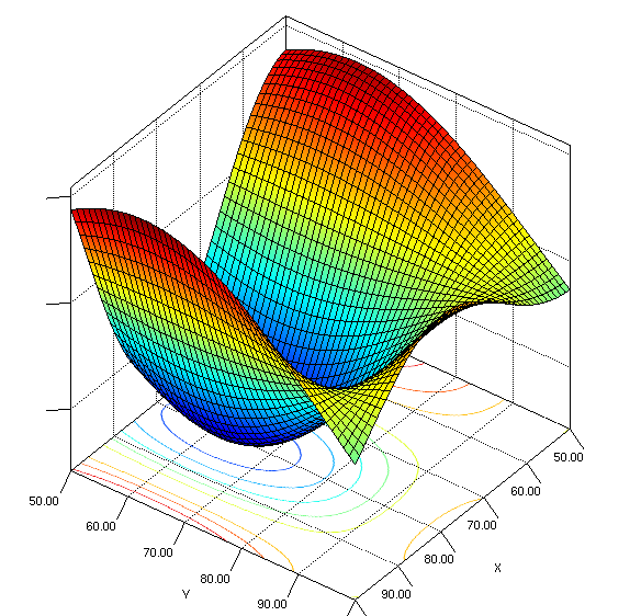
If we consider that the variable plotted on the vertical axis is y, and the values of the 2 variables on the horizontal axes make the input vector X, then our hope is that we are able to find a function f which can approximate the function plotted here. If all the data I collect is such that x₁ belongs to (80,100) and x₂ belongs to (80,100), the learned function will only be able to learn the "yellow-green dipping below" part of the function. Our function will never be able to make good predictions for any values of x₁ or x₂ outside this range.
Therefore, we want to collect data which is representative of all possible movies that we want to make predictions about. Or else (which is often the case), we need to be aware of the limitations of the model we have trained, and the predictions we can make with confidence. The easiest way to do this is to only make predictions about the domain of data we collected the training data from.
We will be scraping data from 2 different movie sources - IMDB and TMDB
IMDB: http://www.imdb.com/
For those unaware, IMDB is the primary source of information about movies on the internet. It is immensely rich with posters, reviews, synopsis, ratings and many other information on every movie. We will use this as our primary data source.
TMDB: https://www.themoviedb.org/
TMDB, or The Movie DataBase, is an open source version of IMDB, with a free to use API that can be used to collect information. You do need an API key, but it can be obtained for free by registering on TMDB.
Note
IMDB gives some information for free through the API, but doesn't release other information about movies. Here, we will keep it legal and only use information given to us for free and legally. However, scraping does reside on the moral fence, so to say. People often scrape data which isn't exactly publicly available for use from websites.
Broad outline of technical steps for data collection
- Sign up for TMDB (themoviedatabase.org), and set up API to scrape movie posters for above movies.
- Set up and work with TMDb to get movie information from their database
- Do the same for IMDb
- Compare the entries of both datasets
Signing up for TMDB and getting set up for getting movie metadata
- Step 1. Head over to tmdb.org and create a new account there by signing up.
- Step 2. Click on your account icon on the top right, then from drop down menu select settings.
- Step 3. Click on API on the left sidebar and then follow instructions to register for an API key.
Using TMDB with the obtained API Key to get movie information
I have made these functions which make things easy. Basically, I'm making use of a library called tmdbsimple which makes TMDB usage even easier. This library was installed at the time of setup.
However, if you want to avoid the library, it is also easy enough to load the API output directly into a dictionary like this without using tmdbsimple:
url = 'https://api.themoviedb.org/3/movie/1581?api_key=' + api_key
data = urllib2.urlopen(url).read()

# create dictionary from string
dataDict = json.loads(data)
While the above functions have been made to make it easy to get genres, posters and ID, all the information that can be accessed can be seen by calling the function get_movie_info().
Getting movie information from IMDB
Now that we know how to get information from TMDB, here's how we can get information about the same movie from IMDB. This makes it possible for us to combine more information, and get a richer dataset. I urge you to try and see what dataset you can make, and go above and beyond the basic things I've done in this tutorial. Due to the differences between the two datasets, you will have to do some cleaning, however both of these datasets are extremely clean and it will be minimal.
A small comparison of IMDB and TMDB
Now that we have both systems running, let's do a very short comparison for the same movie. As we can see, both the systems are correct, but the way they package information is different. TMDB calls it "Science Fiction" and has an ID for every genre, while IMDB calls it "Sci-Fi". Thus, it is important to keep track of these things when making use of both the datasets simultaneously.
Working with multiple movies: Obtaining Top 20 movies from TMDB
We first instantiate an object that inherits from class Movies from TMDB. Then we use the popular() class method to get top movies. To get more than one page of results, the optional page argument lets us see movies from any specified page number.
TMDB doesn't want to make your job as easy as you thought. Why these random numbers? Want to see their genre names? Well, there's the Genre() class for it. Let's convert this list into a nice dictionary to look up genre names from genre IDs!
Section 4. Building a Dataset to Work With
Making use of the same API as before, we will just pull results from the top 50 pages. As mentioned earlier, the "page" attribute of the command top_movies=all_movies.popular() can be used for this purpose.
Please note: Some of the code below will store the data into Python "pickle" files so that it can be read directly from memory, as opposed to being downloaded every time. Once done, you should comment out any code which generated an object that was pickled and is no longer needed.
Pairwise analysis of Movie Genres
As our dataset is multi label, simply looking at the distribution of genres is not sufficient. It might be beneficial to see which genres co-occur, as it might shed some light on inherent biases in our dataset. For example, it would make sense if romance and comedy occur together more often than documentary and comedy. Such inherent biases tell us that the underlying population we are sampling from itself is skewed and not balanced. We may then take steps to account for such problems. Even if we are unable to address the problems, being aware of them is always a good idea.
We pull genres for each movie, and use a function to count occurrences of when two genres occurred together. Let's take a look at the structure we just made. It is a 19×19 structure. Needless to say, this structure counts the number of simultaneous occurrences of genres in the same movie.
The above image shows how often the genres occur together, as a heatmap.
Important thing to notice in the above plot is the diagonal. The diagonal corresponds to self-pairs, i.e. number of times a genre, say Drama occurred with Drama. Which is basically just a count of the total times that genre occurred!
As we can see there are a lot of dramas in the data set — it is also a very unspecific label. There are nearly no documentaries or TV Movies. Horror is a very distinct label, and romance is also not too widely spread.
Delving Deeper into co-occurrence of genres
What we want to do now is to look for nice groups of genres that co-occur, and see if it makes sense to us logically. Intuitively speaking, wouldn't it be fun if we saw nice boxes on the above plot — boxes of high intensity, i.e. genres that occur together and don't occur much with other genres. In some ways, that would isolate the co-occurrence of some genres, and heighten the co-occurrence of others.
While the data may not show that directly, we can play with the numbers to see if this pattern emerges. Using biclustering (SpectralCoclustering from sklearn), we can rearrange the rows and columns to reveal natural groupings.
Looking at the figure, "boxes" or groups of movie genres automatically emerge! Intuitively — Crime, Sci-Fi, Mystery, Action, Horror, Drama, Thriller, etc co-occur. AND, Romance, Fantasy, Family, Music, Adventure, etc co-occur. That makes a lot of intuitive sense, right?
from sklearn.cluster import SpectralCoclustering

model = SpectralCoclustering(n_clusters=5)
model.fit(visGrid)
fit_data = visGrid[np.argsort(model.row_labels_)]
fit_data = fit_data[:, np.argsort(model.column_labels_)]
Based on playing around with the stuff above, we can sort the data into the following genre categories — "Drama, Action, ScienceFiction, exciting (thriller, crime, mystery), uplifting (adventure, fantasy, animation, comedy, romance, family), Horror, History"
Note: that this categorization is subjective and by no means the only right solution. One could also just stay with the original labels and only exclude the ones with not enough data. Such tricks are important to balance the desire to have a rich dataset, while also dealing with the problems of having too many categories.
Interesting Questions
This really should be a place for you to get creative and hopefully come up with better questions than me. Here are some of my thoughts:
- Which actors are bound to a genre, and which can easily hop genres?
- Is there a trend in genre popularity over the years?
- Can you use sound tracks to identify the genre of a movie?
- Are top romance actors higher paid than action heroes?
Building a dataset out of the scraped information
This task is simple, but extremely important. It's basically what will set the stage for the whole project. Given that you have the freedom to cast their own project within the framework I am providing, there are many decisions that you must make to finalize your own version of the project.
As we are working on a classification problem, we need to make two decisions given the data at hand:
- What do we want to predict, i.e. what's our Y?
- What features to use for predicting this Y, i.e. what X should we use?
There are many different options possible, and it comes down to you to decide what's most exciting. I will be picking my own version for the example, but it is imperative that you think this through, and come up with a version which excites you!
As an example, here are some possible ways to frame Y, while still sticking to the problem of genre prediction:
- Assume every movie can have multiple genres, and then it becomes a multi-label classification problem. For example, a movie can be Action, Horror and Adventure simultaneously. Thus, every movie can be more than one genre.
- Make clusters of genres as we did using biclustering, and then every movie can have only 1 genre. This way, the problem is simpler — a multi-class classification problem.
Similarly, for designing our input features i.e. X, you may pick any features you think make sense. For example, the Director of a movie may be a good predictor for genre. OR, you may choose any features designed using algorithms like PCA. Given the richness of IMDB, TMDB and alternate sources like Wikipedia, there is a plethora of options available. Be creative here!
My Implementation
Implementation decisions made:
- The problem is framed here as a multi-label problem explained above.
- We will try to predict multiple genres associated with a movie. This will be our Y.
- We will use 2 different kinds of X — text and images.
- For the text part — Input features being used to predict the genre is a form of the movie's plot available from TMDB using the property 'overview'. This will be our X.
- For the image part — we will use the scraped movie posters as input features.
First, let's identify movies that have overviews. Next few steps are going to be a good example on why data cleaning is important!
Now let's store the genres for these movies in a list that we will later transform into a binarized vector. Binarized vector representation is a very common and important way data is stored/represented in ML. Essentially, it's a way to reduce a categorical variable with n possible values to n binary indicator variables. For example, if sample A has labels 1 and 3, and sample B has label 4, then for every sample, for every possible label, we maintain a 0 or 1 to tell us if a sample has that label or not.
from sklearn.preprocessing import MultiLabelBinarizer
mlb = MultiLabelBinarizer()
Y = mlb.fit_transform(genres)
This is interesting. We started with only 19 genre labels. But the shape for Y is 1666×20 while it should be 1666×19 as there are only 19 genres! Turns out, one genre ID wasn't given to us by TMDB when we asked it for all possible genres. After some digging, I found that this ID corresponds to the genre "Foreign". Such problems are ubiquitous in machine learning, and it is up to us to diagnose and correct them.
So, how do we store this movie overview in a matrix?
Do we just store the whole string? We know that we need to work with numbers, but this is all text. What do we do?!
The way we will be storing the X matrix is called a "Bag of Words" representation. The basic idea of this representation in our context is that we can think of all the distinct words that are possible in the movies' reviews as a distinct object. And then every movie overview can be thought as a "Bag" containing a bunch of these possible objects.
What this means is that, for all the movies that we have the data on, we will first count all the unique words. Say, there's 30,000 unique words. Then we can represent every movie overview as a 30,000×1 vector, where each position in the vector corresponds to the presence or absence of a particular word. If the word corresponding to that position is present in the overview, that position will have 1, otherwise it will be 0.
Are all words equally important?
At the cost of sounding "Animal Farm" inspired, I would say not all words are equally important.
For "The Matrix" a word like "computer" is a stronger indicator of it being a Sci-Fi movie, than words like "who" or "powerful" or "vast". One way computer scientists working with natural language tackled this problem in the past (and it is still used very popularly) is what we call TF-IDF i.e. Term Frequency, Inverse Document Frequency. The basic idea here is that words that are strongly indicative of the content of a single document (every movie overview is a document in our case) are words that appear frequently in that document but rarely in other documents.
The Curse of Dimensionality
This section is strongly borrowing from one of the greatest ML papers I've ever read.
This expression was coined by Bellman in 1961 to refer to the fact that many algorithms that work fine in low dimensions become intractable when the input is high-dimensional.
Now, let's increase the dimensionality i.e. number of dependent variables and see what happens. Say, we have 2 variables x₁ and x₂, same possible values as before — integers between 1 and 100. Now, instead of a line, we'll have a plane with x₁ and x₂ on the two axes. The interesting bit is that instead of 100 possible values of dependent variables like before, we now have 100,000 possible values! Basically, we can make a 100×100 table of possible values of x₁ and x₂. Wow, that increases the sample set we need!
For 3 variables, it would be 100,000,000, and we'd need to sample at 500,000 points. That's already more than the number of data points we have for most training problems we will ever come across.
Basically, as the dimensionality (number of features) of the examples grows, a fixed-size training set covers a dwindling fraction of the input space. Even with a moderate dimension of 100 and a huge training set of a trillion examples, the latter covers only a fraction of about 10⁻¹⁸ of the input space. This is what makes machine learning both necessary and hard.
So, yes, if some words are unimportant, we want to get rid of them and reduce the dimensionality of our X matrix. And the way we will do it is using TF-IDF to identify un-important words. Python lets us do this with just one line of code (And this is why you should spend more time reading maths, than coding!)
from sklearn.feature_extraction.text import TfidfVectorizer
vectorizer = TfidfVectorizer(min_df=10, max_df=0.8)
X = vectorizer.fit_transform(overviews)
We are excluding all words that occur in too many or too few documents, as these are very unlikely to be discriminative. Words that only occur in one document most probably are names, and words that occur in nearly all documents are probably stop words.
So, each movie's overview gets represented by a 1×1365 dimensional vector. Now, we are ready for the kill. Our data is cleaned, hypothesis is set (Overview can predict movie genre), and the feature/output vectors are prepped. Let's train some models!
Section 5. Non-deep, Conventional ML Models
Here is a layout of what we will be doing:
- We will implement two different models
- We will decide a performance metric i.e. a quantitative method to be sure about how well different models are doing
- Discussion of the differences between the models, their strengths, weaknesses, etc.
As discussed earlier, there are a LOT of implementation decisions to be made. Between feature engineering, hyper-parameter tuning, model selection and how interpretable do you want your model to be (Read: Bayesian vs Non-Bayesian approaches) a lot is to be decided. For example, some of these models could be:
- Generalized Linear Models
- SVM
- Shallow (1 Layer, i.e. not deep) Neural Network
- Random Forest
- Boosting
- Decision Tree
The list is endless, and not all models will make sense for the kind of problem you have framed for yourself. Think about which model best fits for your purpose.
For our purposes here, I will be showing the example of 2 very simple models, one picked from each category above:
- SVM
- Multinomial Naive Bayes
Let's start with some feature engineering
Engineering the right features depends on 2 key ideas. Firstly, what is it that you are trying to solve? For example, if you want to guess my music preferences and you try to train a super awesome model while giving it what my height is as input features, you're going to have no luck. On the other hand, giving it my Spotify playlist will solve the problem with any model. So, CONTEXT of the problem plays a role.
Second, you can only represent based on the data at hand. Meaning, if you don't have location data about the user, you simply can't use it no matter how helpful it is.
Once again, the way TF-IDF works — most movie descriptions have the word "The" in it. Obviously, it doesn't tell you anything special about it. So weightage should be inversely proportional to how many movies have the word in their description. This is the IDF part. On the other hand, for the movie Interstellar, if the description has the word "Space" 5 times, and "wormhole" 2 times, then it's probably more about Space than about wormhole. Thus, "space" should have a high weightage. This is the TF part.
Let's divide our X and Y matrices into train and test split. We train the model on the train split, and report the performance on the test split. Think of this like the questions you do in the problem sets v/s the exam. Of course, they are both (assumed to be) from the same population of questions. And doing well on Problem Sets is a good indicator that you'll do well in exams, but really, you must test before you can make any claims about you knowing the subject.
from sklearn.multiclass import OneVsRestClassifier
from sklearn.svm import LinearSVC
from sklearn.naive_bayes import MultinomialNB
from sklearn.model_selection import train_test_split

X_train, X_test, Y_train, Y_test = train_test_split(X, Y, test_size=0.2)

# SVM Model
svm = OneVsRestClassifier(LinearSVC())
svm.fit(X_train, Y_train)
svm_predictions = svm.predict(X_test)

# Naive Bayes Model
nb = OneVsRestClassifier(MultinomialNB())
nb.fit(X_train, Y_train)
nb_predictions = nb.predict(X_test)
As you can see, the performance is by and large poorer for movies which are less represented like War and Animation, and better for categories like Drama.
For multi-label systems, we often keep track of performance using "Precision" and "Recall". Precision tells us how many of the positively predicted labels are actually correct, and recall tells us how many of the actual positive labels were correctly predicted.
The average precision and recall scores for our samples are pretty good! Models seem to be working! Also, we can see that the Naive Bayes outperforms SVM. I strongly suggest you to go read about Multinomial Bayes and think about why it works so well for "Document Classification", which is very similar to our case as every movie overview can be thought of as a document we are assigning labels to.
Section 6. Deep Learning: An Intuitive Overview
The above results were good, but it's time to bring out the big guns. So first and foremost, let's get a very short idea about what's deep learning. This is for people who don't have background in this — it's high level and gives just the intuition.
As described above, the two most important concepts in doing good classification (or regression) are to 1) use the right representation which captures the right information about the data which is relevant to the problem at hand, and 2) using the right model which has the capability of making sense of the representation fed to it.
While for the second part we have complicated and powerful models that we have studied at length, we don't seem to have a principled, mathematical way of doing the first part — i.e. representation. What we did above was to see "what makes sense", and go from there. That is not a good approach for complex data or complex problems. Is there some way to automate this? Deep Learning does just this.
To emphasize the importance of representation in the complex tasks we usually attempt with Deep Learning, let me talk about the original problem which made it famous. The paper is often referred to as the "Imagenet Challenge Paper", and it was basically working on object recognition in images. Let's try to think about an algorithm that tries to detect a chair.
If I ask you to "Define" a chair, how would you? — Something with 4 legs?
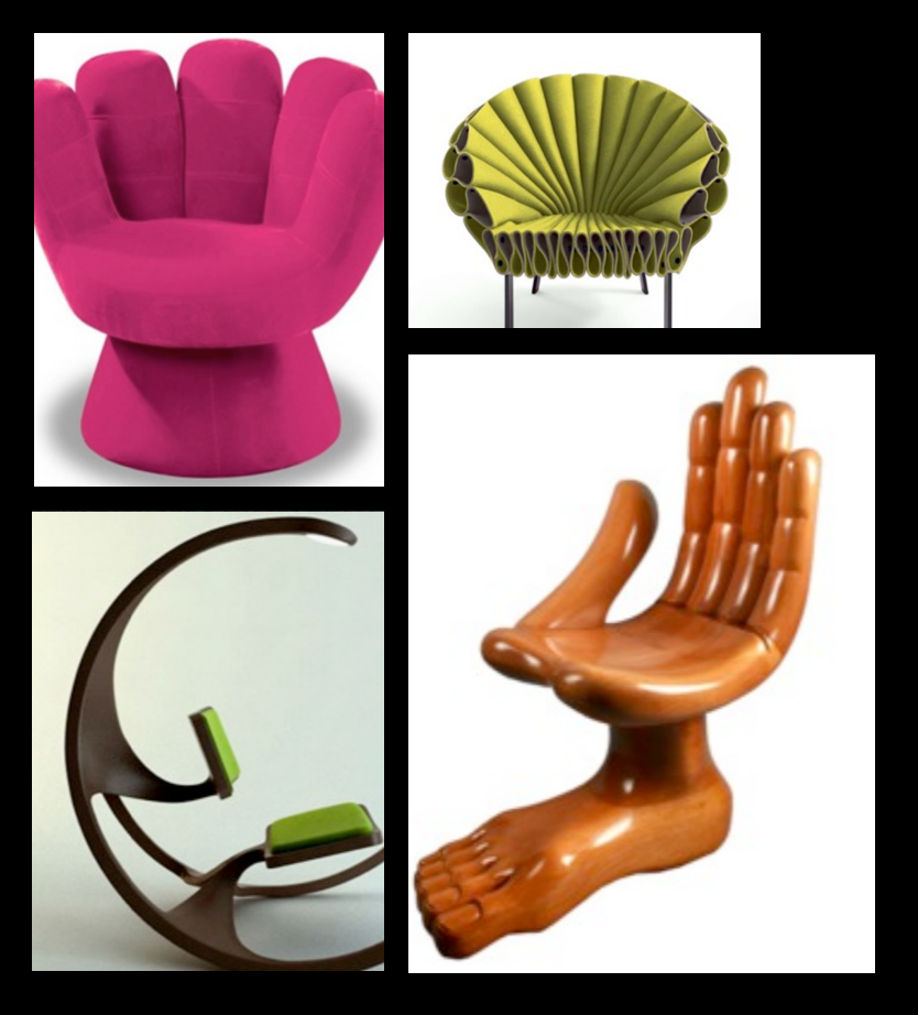
All are chairs, none with 4 legs. (Pic Credit: Zoya Bylinskii)
How about some surface that we sit on then?
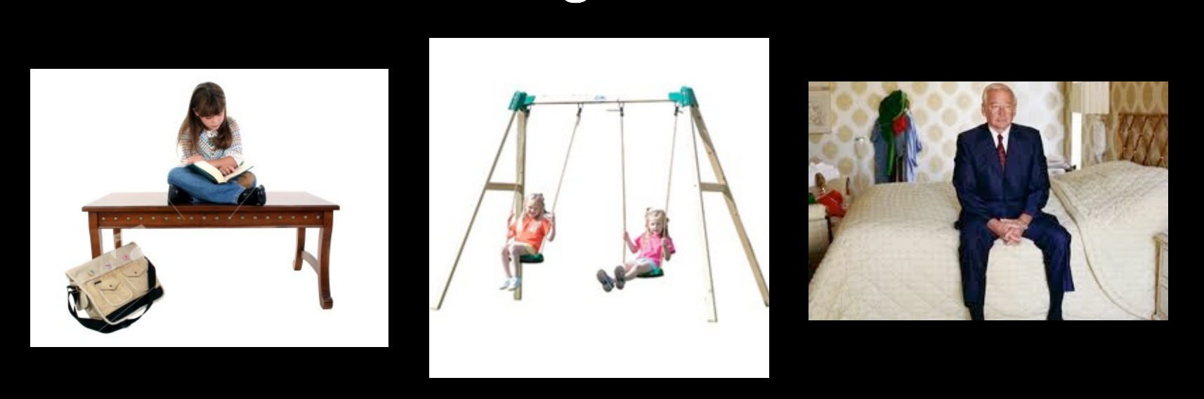
All are surfaces we sit on, none are chairs. (Pic Credit: Zoya Bylinskii)
Clearly, these definitions won't work and we need something more complicated. Sadly, we can't come up with a simple text rule that our computer can search for! And we take a more principled approach.
The "Deep" in deep learning comes from the fact that it was conventionally applied to Neural Networks. Neural Networks, as we all know, are structures organized in layers. Layers of computations. Why do we need layers? Because these layers can be seen as sub-tasks that we do in the complicated task of identifying a chair. It can be thought as a hierarchical break down of a complicated job into smaller sub-tasks.
Mathematically, each layer acts like a space transformation which takes the pixel values to a high dimensional space. When we start out, every pixel in the image is given equal importance in our matrix. With each layer, convolution operations give some parts more importance, and some lesser importance. In doing so, we transform our images to a space in which similar looking objects/object parts are closer (We are basically learning this space transformation in deep learning, nothing else).
What exactly was learnt by these neural networks is hard to know, and an active area of research. But one very crude way to visualize what it does is to think like: It starts by learning very generic features in the first layer — something as simple as vertical and horizontal lines. In the next layer, it learns that if you combine the vectors representing vertical and horizontal vectors in different ratios, you can make all possible slanted lines. Next layer learns to combine lines to form curves — say, something like the outline of a face. These curves come together to form 3D objects. And so on. Building sub-modules, combining them in the right way which can give it semantics.
So, in a nutshell, the first few layers of a "Deep" network learn the right representation of the data, given the problem (which is mathematically described by your objective function trying to minimize difference between ground truth and predicted labels). The last layer simply looks how close or far apart things are in this high dimensional space.
Hence, we can give any kind of data a high dimensional representation using neural networks. Below we will see high dimensional representations of both words in overviews (text) and posters (image). Let's get started with the posters i.e. extracting visual features from posters using deep learning.
Section 7. Deep Learning for Predicting Genre from Poster
Once again, we must make an implementation decision. This time, it has more to do with how much time are we willing to spend in return for added accuracy. We are going to use here a technique that is commonly referred to as Pre-Training in Machine Learning Literature.
Instead of me trying to re-invent the wheel here, I am going to borrow this short section on pre-training from Stanford University's lecture on CNN's. To quote:
"In practice, very few people train an entire Convolutional Network from scratch (with random initialization), because it is relatively rare to have a dataset of sufficient size. Instead, it is common to pretrain a ConvNet on a very large dataset (e.g. ImageNet, which contains 1.2 million images with 1000 categories), and then use the ConvNet either as an initialization or a fixed feature extractor for the task of interest."
There are three broad ways in which transfer learning or pre-training can be done. The way we are going to about it is by using a pre-trained, released ConvNet as feature extractor. Take a ConvNet pretrained on ImageNet (a popular object detection dataset), remove the last fully-connected layer. After removing the last layer, what we have is just another neural network — a stack of space transformations. But, originally the output of this stack can be pumped into a single layer which can classify the image into categories like Car, Dog, Cat and so on.
What this means is that in the space this stack transforms the images to, all images which contain a "dog" are closer to each other, and all images containing a "cat" are closer. Thus, it is a meaningful space where images with similar objects are closer.
Think about it — now if we pump our posters through this stack, it will embed them in a space where posters which contain similar objects are closer. This is a very meaningful feature engineering method! While this may not be ideal for genre prediction, it might be quite meaningful. For example, all posters with a gun or a car are probably action. While a smiling couple would point to romance or drama.
This way, we can start off with something strong, and then build on top. We pump our images through the pre-trained network to extract the visual features from the posters. Then, using these features as descriptors for the image, and genres as the labels, we train a simpler neural network from scratch which learns to do simply classification on this dataset.
Deep Learning to extract visual features from posters
The basic problem here we are answering is: can we use the posters to predict genre? First check — Does this hypothesis make sense? Yes. Because that's what graphic designers do for a living. They leave visual cues to semantics. They make sure that when we look at the poster of a horror movie, we know it's not a happy image. Things like that. Can our deep learning system infer such subtleties? Let's find out!
For visual features, we can use a pre-trained network made available to us from the Visual Geometry Group at Oxford University, one of the most popular methods. This is called the VGG-net. Mathematically, it's just a space transformation in the form of layers. So, we simply need to perform this chain of transformations on our image. Keras is a library that makes it very easy for us to do this.
from keras.applications.vgg16 import VGG16
from keras.preprocessing import image
from keras.applications.vgg16 import preprocess_input
import numpy as np

model = VGG16(weights='imagenet', include_top=False)

# For each movie poster:
img = image.load_img(img_path, target_size=(224, 224))
x = image.img_to_array(img)
x = np.expand_dims(x, axis=0)
x = preprocess_input(x)
features = model.predict(x)
The final movie poster set for which we have all the information we need is 1265 movies. The VGG features are reshaped to be in the shape (1, 25088) and we finally obtain a matrix of shape (1265, 25088).
Training a simple neural network model using these VGG features
Now, we create our own Keras neural network to use the VGG features and then classify movie genres. Keras makes this super easy.
Neural network architectures have gotten complex over the years. But the simplest ones contain very standard computations organized in layers. Given the popularity of some of these, Keras makes it as easy as writing out the names of these operations in a sequential order.
Important Question: Why do we need activation functions?
Sometimes, we tend to get lost in the jargon and confuse things easily, so the best way to go about this is getting back to our basics.
Don't forget what the original premise of machine learning (and thus deep learning) is — IF the input and output are related by a function y=f(x), then if we have x, there is no way to exactly know f unless we know the process itself. However, machine learning gives you the ability to approximate f with a function g, and the process of trying out multiple candidates to identify the function g best approximating f is called machine learning.
Deep learning simply tries to expand the possible kind of functions that can be approximated using the above mentioned machine learning paradigm. Roughly speaking, if the previous model could learn say 10,000 kinds of functions, now it will be able to learn say 100,000 kinds.
If you want to know the mathematics of it, go read about VC dimension and how more layers in a network affect it. But I will avoid the mathematics here and rely on your intuition to believe me when I say that not all data can be classified correctly into categories using a linear function. So, we need our deep learning model to be able to approximate more complex functions than just a linear function.
Now, let's come to the non-linearity bit. Imagine a linear function y=2x+3, and another one y=4x+7. What happens if I pool them and take an average? I get another linear function y=3x+5. So instead of doing those two computations separately and then averaging it out, I could have just used the single linear function y=3x+5. This is exactly what will happen if you don't have non-linearities in your nodes.
It simply follows from the definition of a linear function: if you take two linear functions AND take a linear combination of them (which is how we combine the outputs of multiple nodes of a network), you are BOUND to get a linear function because f(x)+g(x)=mx+b+nx+c=(m+n)x+(b+c).
And you could in essence replace your whole network by a simple matrix transformation. In a nutshell, you'll only be trying to learn a linear approximation for original function f. Adding non-linearities ensures that you can learn more complex functions by approximating every non-linear function as a LINEAR combination of a large number of non-linear functions.
Let's train our model then, using the features we extracted from VGG net
The model we will use has just 1 hidden layer between the VGG features and the final output layer. The simplest neural network you can get. An image goes into this network with the dimensions (1, 25088), the first layer's output is 1024 dimensional. This hidden layer output undergoes a pointwise RELU activation. This output gets transformed into the output layer of 20 dimensions. It goes through a sigmoid.
The sigmoid, or the squashing function as it is often called, is a function which squashes numbers between 0 and 1. What are you reminded of when you think of numbers between 0 and 1? Right, probability. By squashing the score of each of the 20 output labels between 0 and 1, sigmoid lets us interpret their scores as probabilities. Then, we can just pick the classes with the top 3 or 5 probability scores as the predicted genres for the movie poster!
from keras.models import Sequential
from keras.layers import Dense, Activation
from keras import optimizers

model_visual = Sequential([
    Dense(1024, input_shape=(25088,)),
    Activation('relu'),
    Dense(256),
    Activation('relu'),
    Dense(20),
    Activation('sigmoid'),
])

opt = optimizers.rmsprop(lr=0.0001, decay=1e-6)
model_visual.compile(optimizer=opt,
              loss='binary_crossentropy',
              metrics=['accuracy'])

model_visual.fit(X_train, Y_train, epochs=100, batch_size=50)
Section 8. Deep Learning to Get Textual Features
Let's do the same thing as above with text now.
We will use an off the shelf representation for words — Word2Vec model. Just like VGGnet before, this is a model made available to get a meaningful representation. As the total number of words is small, we don't even need to forward propagate our sample through a network. Even that has been done for us, and the result is stored in the form of a dictionary. We can simply look up the word in the dictionary and get the Word2Vec features for the word.
from gensim import models

model2 = models.KeyedVectors.load_word2vec_format(
    'GoogleNews-vectors-negative300.bin', binary=True)

# Get the Word2Vec representation of a word:
print(model2['king'].shape)   # (300,)
print(model2['dog'].shape)    # (300,)
This way, we can represent the words in our overviews using this Word2Vec model. And then, we can use that as our X representations. So, instead of count of words, we are using a representation which is based on the semantic representation of the word. Mathematically, each word went from 3-4 dimensional (the length) to 300 dimensions!
For the same set of movies above, let's try and predict the genres from the deep representation of their overviews!
Even without much tuning of the above model, these results are able to beat our previous results.
Note — I got accuracies as high as 78% when doing classification using plots scraped from Wikipedia. The large amount of information was very suitable for movie genre classification with a deep model. I strongly suggest you try playing around with architectures.
Section 9. Upcoming Tutorials and Acknowledgements
Congrats! This is the end of our pilot project! Needless to say, a lot of the above content may be new to you, or may be things that you know very well. If it's the former, I hope this tutorial would have helped you. If it is the latter and you think I wrote something incorrect or that my understanding can be improved, feel free to create a GitHub issue so that I can correct it!
I would like to thank a few of my friends who had an indispensable role to play in me making this tutorial. Firstly, Professor Hanspeter Pfister and Verena Kaynig at Harvard, who helped guide this tutorial/project and scope it. Secondly, my friends Sahil Loomba and Matthew Tancik for their suggestions and editing the material and the presentation of the storyline. Thirdly, Zoya Bylinskii at MIT for constantly motivating me to put in my effort into this tutorial. Finally, all others who helped me feel confident enough to take up this task and to see it till the end. Thanks all of you!